Tool Demos
GradDog includes tools to allow users to easily perform common actions on scalar functions related to their first derivatives. These tools also provide a skeleton for users who desire to write their own tools using GradDog for differentiation.
First, import the full graddog module (recommended alias: gd), the functions from the functions module:
import graddog as gd
from graddog.functions import sin, cos, tan, exp, log
Then, create the function you would like to use (See this link for more information on creating your own Python functions):
def quadratic(x):
     a=4
     xoffset = 3
     yoffset = 0
     return a*(x-xoffset)**2 + yoffset
All tools in the tools.py module also take in the lower and upper limits of the x-interval on which you’d like to evaluate the derivative. More detail on each of their inputs and outputs is provided below.
plot_derivative:
The plot_derivative tool plots the derivative of the provided function over a given interval. This is a numerical method and therefore includes an n_pts parameter that can be increased to improve resolution or decreased to improve speed. The default value is 100, which suffices for most simple plots.
Inputs:
function[function]: the function of which you’d like to plot the derivative (must only take single input)
xmin: lower bound on which to calculate derivative
xmax: upper bound on which to calculate derivative
n_pts [int](Default: 100): how many points to use when evaluating derivative (more = better resolution but slower)
figsize [tuple](Default: (6,6)): figsize in inches (see matplotlib documentation)
xlabel [string](Default: ‘x’): Label for x axis of plot
ylabel [string](Default: ‘y’): Label for y axis of plot
plotTitle [string](Default: ‘Derivative’): Label for title of plot
Outputs:
xs: the array of linearly spaced x values between xmin and xmax
ys: the derivative evaluated at the values in xs
Example:
xs, ys = plot_derivative(quadratic, 0, 5)
find_extrema_first_order:
The find_extrema_first_order tool locates the point where the derivative is closest to zero on the given interval.
Inputs:
function[function]: the function of which you’d like to plot the derivative. (one scalar input)
xmin: lower bound on which to calculate derivative
xmax: upper bound on which to calculate derivative
n_pts [int](Default: 100): how many points to use when evaluating derivative (more = better resolution but slower)
tolerance [float](Default: 1e-10): how close to zero should a value be before it’s considered an extrema?
Outputs: If it can locate your extrema exactly, it will return only the x value(s) of the extrema. If not it will return:
xs: a tuple containing the two x values between which the extrema is located
To locate the extrema on the interval (-10,10) for the quadratic function defined above Example:
x_extr = find_extrema_firstorder(quadratic, -10, 10)
In this case, the function fails to find the precise extrema, but instead returns a tuple of x values that the extrema is between.
Example:
def fun(x):
     return 3*x**4 - 6*x**3
xs_EX = find_extrema_firstorder(fun, -2, 4)
In this case, the function finds the exact extrema, so it returns only that value. If there is more than one point in the given interval that is lower than the tolerance value, it will return xvalues for all points.
find_increasing
The find_increasing tool locates the region on a given interval where the function is increasing.
Inputs:
function[function]: the function that you want to locate increasing regions on (one scalar input)
xmin: lower bound of interval
xmax: upper bound of interval
n_pts (default = 100): how many points to use when evaluating derivative (more = better resolution but slower)
Outputs:
xs: the x values where the function is increasing
ys: the y values where the function is increasing
To locate the increasing region on the interval (-5,5) for the quadratic function defined above Example:
xinc, yinc = find_increasing(quadratic, -5, 5)
find_decreasing:
The find_decreasing tool locates the region on a given interval where the function is decreasing.
Inputs:
function[function]: the function that you want to locate decreasing regions on (one scalar input)
xmin: lower bound of interval
xmax: upper bound of interval
n_pts (default = 100): how many points to use when evaluating derivative (more = better resolution but slower)
Outputs:
xs: the x values where the function is decreasing
ys: the y values where the function is decreasing
To locate the decreasing region on the interval (-5,5) for the quadratic function defined above Example:
xdec, ydec = find_decreasing(quadratic, -5, 5)
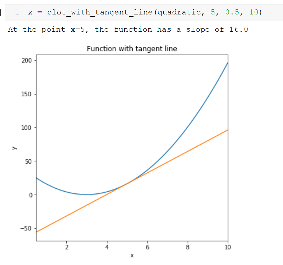
plot_with_tangent_line:
The plot_with_tangent_line tool plots the provided function with a tangent line at a specified point.
Inputs:
function[function]: the function you’d like to plot.
xtangent: value at which you want the tangent line to intersect the function
xmin: lower bound on which to plot
xmax: upper bound on which to plot
n_pts [int](Default: 100): how many points to use when plotting function (more = better resolution but slower)
figsize [tuple](Default: (6,6)): figsize in inches (see matplotlib documentation)
xlabel [string](Default: ‘x’): Label for x axis of plot
ylabel [string](Default: ‘y’): Label for y axis of plot
plotTitle [string](Default: ‘Derivative’): Label for title of plot
Outputs:
xs: the array of linearly spaced x values between xmin and xmax
ys: the derivative evaluated at the values in xs
To plot a function and its tangent line at x=1 on the interval (-2,2):
def f(x):
    return 4*x**3 - 5*x
xs, ys = plot_with_tangent_line(f, 1, -2, 2)